Multi-dimensional fitting

GModelFit.jl supports multi-dimensional data fitting, namely the case where both the model and the empirical measures are expressed as a function of an N-dimensional domain.

Example in 2D

using GModelFit

model = Model(:background => GModelFit.OffsetSlope(0, 0, 0., 0.5, 1.),
              :psf => GModelFit.Gaussian(100., 0., 0., 1, 0.3, 15),
			  :main => SumReducer(:background, :psf))

dom = CartesianDomain(-5:0.25:5, -4:0.25:4)
data = GModelFit.mock(Measures, model, dom)

bestfit, fsumm = fit(model, data)

(Components:
╭───────────────┬────────────────┬───────┬─────────────┬───────────┬───────────┬───────────┬─────────╮
│   Component   │      Type      │ #Free │ Eval. count │    Min    │    Max    │   Mean    │ NaN/Inf │
├───────────────┼────────────────┼───────┼─────────────┼───────────┼───────────┼───────────┼─────────┤
│ main          │ SumReducer     │       │ 192         │    -6.416 │     51.05 │     1.294 │ 0       │
│ ├─╴background │ OffsetSlope_2D │ 3     │ 80          │    -6.416 │      6.64 │    0.1119 │ 0       │
│ └─╴psf        │ Gaussian_2D    │ 6     │ 132         │ 3.526e-61 │     50.94 │     1.182 │ 0       │
╰───────────────┴────────────────┴───────┴─────────────┴───────────┴───────────┴───────────┴─────────╯

Parameters:
╭────────────┬────────────────┬─────────┬──────────┬────────────┬───────────┬────────┬───────╮
│ Component  │      Type      │ Param.  │  Range   │   Value    │  Uncert.  │ Actual │ Patch │
├────────────┼────────────────┼─────────┼──────────┼────────────┼───────────┼────────┼───────┤
│ background │ OffsetSlope_2D │ offset  │ -Inf:Inf │    0.1119  │   0.08314 │        │       │
│            │                │ x0      │ -Inf:Inf │         0  │  (fixed)  │        │       │
│            │                │ y0      │ -Inf:Inf │         0  │  (fixed)  │        │       │
│            │                │ slopeX  │ -Inf:Inf │    0.5029  │    0.0269 │        │       │
│            │                │ slopeY  │ -Inf:Inf │     1.003  │   0.03336 │        │       │
├────────────┼────────────────┼─────────┼──────────┼────────────┼───────────┼────────┼───────┤
│ psf        │ Gaussian_2D    │ norm    │ 0:Inf    │     99.96  │     2.225 │        │       │
│            │                │ centerX │ -Inf:Inf │ -0.0004618 │   0.02134 │        │       │
│            │                │ centerY │ -Inf:Inf │ -0.001919  │  0.008558 │        │       │
│            │                │ sigmaX  │ 0:Inf    │     1.004  │   0.02174 │        │       │
│            │                │ sigmaY  │ 0:Inf    │     0.311  │  0.006722 │        │       │
│            │                │ angle   │ -Inf:Inf │      14.5  │    0.5891 │        │       │
╰────────────┴────────────────┴─────────┴──────────┴────────────┴───────────┴────────┴───────╯
, Fit summary: #data: 1353, #free pars: 9, red. fit stat.: 0.94008, status: OK      
)

the results can be displayed with Gnuplot.jl as follows:

using Gnuplot

# Plot the model...
@gsp "set palette" axes(dom, 1) axes(dom, 2) model(dom) "w pm3d notit"

# ... and the data
@gsp :- axes(dom, 1) axes(dom, 2) values(data) "w dots notit lc rgb 'gray'"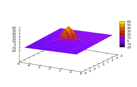

Example in 3D

using GModelFit

dom = CartesianDomain(-5:0.1:5, -5:0.1:5, -5:0.1:5)
model = Model(:source => @fd (x, y, z, cx=0., cy=0., cz=0.) -> @. sqrt((x-cx)^2 + (y-cy)^2 + (z-cz)^2))
data = GModelFit.mock(Measures, model, dom)
bestfit, fsumm = fit(model, data)

Nfree=3, evaluations: 50    Time: 0:00:00 (10.41 ms/it)
   fitstat: 1.000063477180244


Nfree=3, evaluations: 50    Time: 0:00:00 (10.66 ms/it)
(Components:
╭───────────┬───────┬───────┬─────────────┬───────────┬───────────┬───────────┬─────────╮
│ Component │ Type  │ #Free │ Eval. count │    Min    │    Max    │   Mean    │ NaN/Inf │
├───────────┼───────┼───────┼─────────────┼───────────┼───────────┼───────────┼─────────┤
│ source    │ FComp │ 3     │ 51          │  0.001115 │     8.661 │     4.851 │ 0       │
╰───────────┴───────┴───────┴─────────────┴───────────┴───────────┴───────────┴─────────╯

Parameters:
╭───────────┬───────┬────────┬──────────┬────────────┬───────────┬────────┬───────╮
│ Component │ Type  │ Param. │  Range   │   Value    │  Uncert.  │ Actual │ Patch │
├───────────┼───────┼────────┼──────────┼────────────┼───────────┼────────┼───────┤
│ source    │ FComp │ cx     │ -Inf:Inf │  0.001033  │ 0.0008206 │        │       │
│           │       │ cy     │ -Inf:Inf │ -0.0001938 │ 0.0008206 │        │       │
│           │       │ cz     │ -Inf:Inf │ 0.0003712  │ 0.0008206 │        │       │
╰───────────┴───────┴────────┴──────────┴────────────┴───────────┴────────┴───────╯
, Fit summary: #data: 1030301, #free pars: 3, red. fit stat.: 1.0001, status: OK      
)

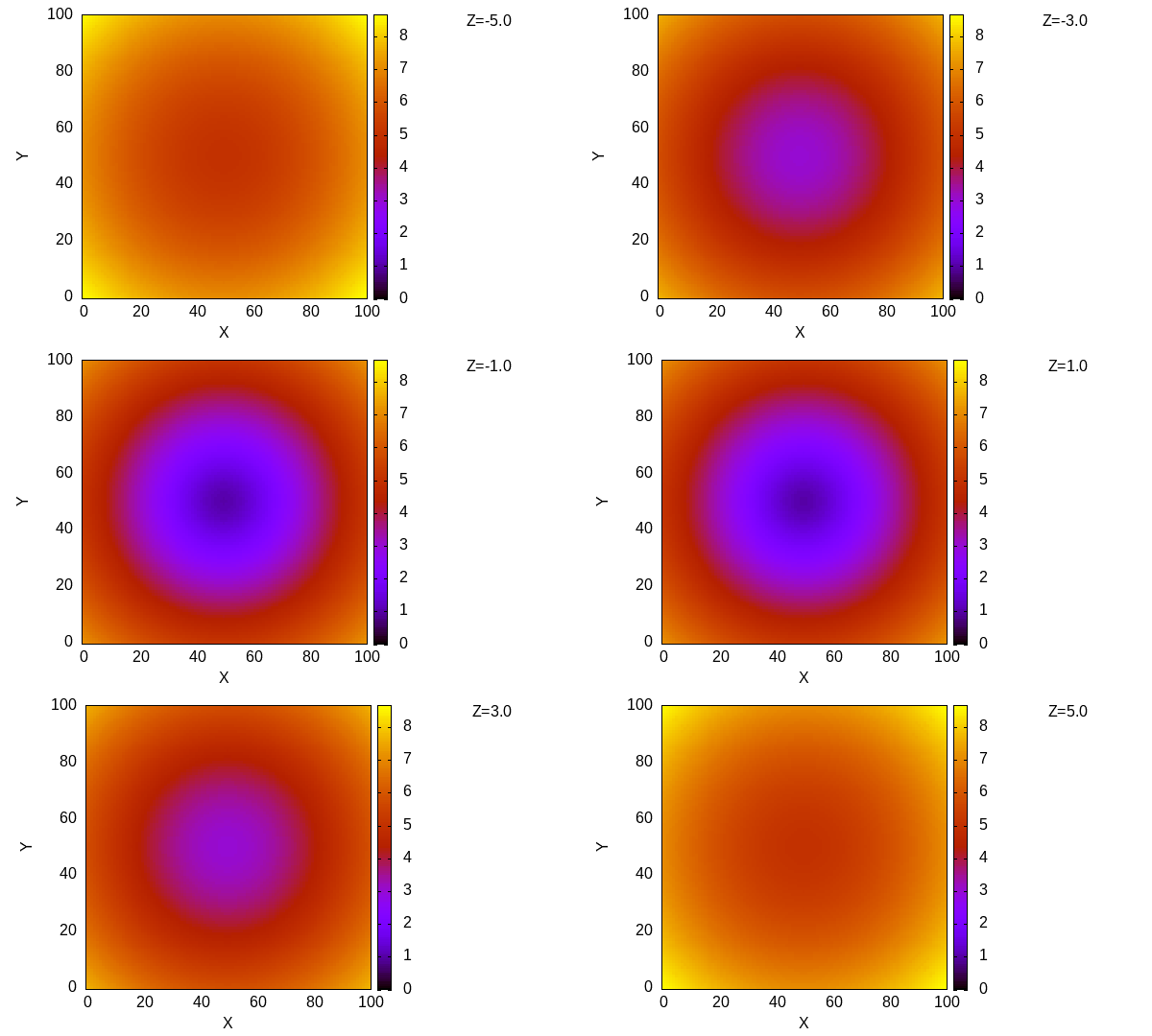
and plot the best-fit model with:

using Gnuplot

m = bestfit()
@gp "set autoscale fix" "set key out" "set size ratio -1" xlab="X" ylab="Y" :-
for i in 1:size(m)[3]
	@gp :- i m[i, :, :] "w image t 'Z=$(string(axes(dom, 3)[i]))'" cbr=extrema(m) :-
end
@gp

"assets/animation.gif"