GModelFit.jl
A model fitting framework for Julia.

GModelFit.jl is a general purpose, data-driven model fitting framework for Julia.
It provides the basic tools to define, interactively manipulate and efficiently evaluate a (possibly very complex) model, and to fit the latter to empirical data. The main functionalities are:
- it handles datasets of any dimensionality;
- the syntax is very simple and concise as it resembles the indexing for dictionaries and the field access for structs. The most relevant functions are the self-explanatory
fit()and the object constructors (see Main functionalities); - the fitting model is evaluated on a user defined domain, and is the result of a combination of model components or mathematical expressions (in the form of lambda functions), or any arbitrary mixture of the two;
- it provides several ready-to-use Built-in components, and it also allows to define new components to suit specific needs (Custom components);
- all components results are cached so that repeated evaluations with the same parameter values do not involve further calculations (memoization);
- model parameters can be fixed to a specific value, limited in an interval, and/or be dynamically linked (patched) to the values of other parameters (see Parameter constraints);
- multiple data sets can be fitted simultaneously against different models whose parameters can be patched (see Multi-dataset fitting);
- it supports different minimizers (LsqFit and CMPFit), both aimed to carry out non-linear least squares minimization (see Minimizers);
- it provides facilities for interactive fitting and quick plotting (see Quick plot (1D)).
The fitting process involves the automatic variation of the parameter values, subject to the user defined constraints, until the differences between the evaluated model and the empirical data are minimized. The implementation details depends on the chosen minimizer. The purpose of GModelFit.jl is thus to act as an interface between the high-level model definition and manipulation (facing the user), and the low-level implementation details (facing the minimizer).
Installation
In the Julia REPL type:
julia> ]add GModelFitThe ] character starts the Julia package manager. Hit backspace key to return to Julia prompt.
In order to easily visualize the outcomes of 1D analysis you may be interested in installing also Gnuplot.jl:
julia> ]add GnuplotWorkflow
The typical workflow to use GModelFit.jl is as follows:
- Wrap empirical data domain and measures into one (ore more)
DomainandMeasuresobject(s); - Create a
Modelobject by providing components or mathematical expressions, each representing a specific aspect of the theoretical model; - Optionally set initial guess parameter values and/or constraints between model parameters;
- Fit the model against the data and inspect the results;
- If needed, modify the model and repeat the fitting process;
- Exploit the results and outputs.
A very simple example showing the above workflow is:
using GModelFit

# Prepare vectors with domain points, empirical measures and associated
# uncertainties
x    = [0.1, 1.1, 2.1, 3.1, 4.1]
meas = [6.29, 7.27, 10.41, 18.67, 25.3]
unc  = [1.1, 1.1, 1.1, 1.2, 1.2]

# Prepare Domain and Measures objects
dom  = Domain(x)
data = Measures(dom, meas, unc)

# Create a model using an explicit mathematical expression, and provide the
# initial guess values:
model = Model(@fd (x, a2=1, a1=1, a0=5) -> (a2 .* x.^2  .+  a1 .* x  .+  a0))

# Fit model to the data
bestfit, stats = fit(model, data)
The GModelFit.jl package implements a show method for many of the data types involved, hence the above code results in the following output:
(Components:
╭───────────┬───────┬───────┬─────────────┬───────────┬───────────┬───────────┬─────────╮
│ Component │ Type  │ #Free │ Eval. count │ Min       │ Max       │ Mean      │ NaN/Inf │
├───────────┼───────┼───────┼─────────────┼───────────┼───────────┼───────────┼─────────┤
│ main      │ FComp │ 3     │ 77          │     6.088 │     25.84 │     13.56 │ 0       │
╰───────────┴───────┴───────┴─────────────┴───────────┴───────────┴───────────┴─────────╯

Parameters:
╭───────────┬───────┬────────┬──────────┬───────────┬───────────┬────────┬───────╮
│ Component │ Type  │ Param. │ Range    │ Value     │ Uncert.   │ Actual │ Patch │
├───────────┼───────┼────────┼──────────┼───────────┼───────────┼────────┼───────┤
│ main      │ FComp │ a2     │ -Inf:Inf │     1.201 │    0.3051 │        │       │
│           │       │ a1     │ -Inf:Inf │    -0.106 │     1.317 │        │       │
│           │       │ a0     │ -Inf:Inf │     6.087 │     1.142 │        │       │
╰───────────┴───────┴────────┴──────────┴───────────┴───────────┴────────┴───────╯
, Fit results: #data: 5, #free pars: 3, red. fit stat.:     1.0129, Status: OK
)
showing the best fit parameter values and the associated uncertaintites, as well as a few statistics concerning the fitting process.
If not saitisfied with the result you may, for instance, change the initial value for a parameter and re-run the fit:
model[:main].a0.val = 5
bestfit, stats = fit(model, data)
Once done, you may plot the data and the best fit model with a plotting framework of your choice. E.g., with Gnuplot.jl:
using Gnuplot
@gp coords(dom) values(data) uncerts(data) "w yerr t 'Data'" :-
@gp :- coords(dom) bestfit() "w l t 'Best fit model'"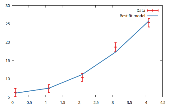
Also, you can easily access the numerical results for further analysis, e.g.:
println("Best fit value for the offset parameter: ",
	bestfit[:main].a0.val, " ± ",
	bestfit[:main].a0.unc, "\n",
	"Reduced χ^2: ", stats.fitstat)
Best fit value for the offset parameter: 6.0869734863133 ± 1.1419446421923485
Reduced χ^2: 1.0128724404973972The above example is definitely a simple one, but more complex ones follow essentially the same workflow.