Built-in components

The GModelFit.jl provides several built-in components which may be used to build arbitrarily complex models.

OffsetSlope

An offset and slope component for 1D and 2D domains.

The constructors are defined as follows:

• 1D: GModelFit.OffsetSlope(offset, x0, slope);
• 2D: GModelFit.OffsetSlope(offset, x0, y0, slopeX, slopeY);

The parameters are:

• 1D:
  • offset::Parameter: a global offset;
  • x0::Parameter: the X coordinate of the point where the component equals offset. This parameter is fixed by default;
  • slope::Parameter: the slope of the linear function;
• 2D:
  • offset::Parameter: a global offset;
  • x0::Parameter: the X coordinate of the point where the component equals offset. This parameter is fixed by default;
  • y0::Parameter: the Y coordinate of the point where the component equals offset. This parameter is fixed by default;
  • slopeX::Parameter (only 2D): the slope of the plane along the X direction;
  • slopeY::Parameter (only 2D): the slope of the plane along the Y direction;

Example

using GModelFit

# Define a linear model using the OffsetSlope component
model = Model(:linear => GModelFit.OffsetSlope(2, 0, 0.5))

# Fit model against data
data = Measures([4.01, 7.58, 12.13, 19.78, 29.04], 0.4)
bestfit, stats = fit(model, data)

(Components:
╭───────────┬────────────────┬───────┬─────────────┬───────────┬───────────┬───────────┬─────────╮
│ Component │ Type           │ #Free │ Eval. count │ Min       │ Max       │ Mean      │ NaN/Inf │
├───────────┼────────────────┼───────┼─────────────┼───────────┼───────────┼───────────┼─────────┤
│ linear    │ OffsetSlope_1D │ 2     │ 42          │     2.056 │     26.96 │     14.51 │ 0       │
╰───────────┴────────────────┴───────┴─────────────┴───────────┴───────────┴───────────┴─────────╯

Parameters:
╭───────────┬────────────────┬────────┬──────────┬───────────┬───────────┬────────┬───────╮
│ Component │ Type           │ Param. │ Range    │ Value     │ Uncert.   │ Actual │ Patch │
├───────────┼────────────────┼────────┼──────────┼───────────┼───────────┼────────┼───────┤
│ linear    │ OffsetSlope_1D │ offset │ -Inf:Inf │     -4.17 │     2.361 │        │       │
│           │                │ x0     │ -Inf:Inf │         0 │  (fixed)  │        │       │
│           │                │ slope  │ -Inf:Inf │     6.226 │    0.7119 │        │       │
╰───────────┴────────────────┴────────┴──────────┴───────────┴───────────┴────────┴───────╯
, Fit results: #data: 5, #free pars: 2, red. fit stat.:     31.671, Status: OK      
)

The best fit parameter values can be retrieved with:

println("Best fit values:")
println("b:  ", bestfit[:linear].offset.val, " ± ", bestfit[:linear].offset.unc)
println("m:  ", bestfit[:linear].slope.val , " ± ", bestfit[:linear].slope.unc)

Best fit values:
b:  -4.1699999993610115 ± 2.3609709866629576
m:  6.225999999809595 ± 0.7118595367099604

A similar example in 2D is as follows:

using GModelFit

# Define a linear model using the OffsetSlope component
model = Model(:plane => GModelFit.OffsetSlope(2, 0, 0, 0.5, 0.5))

# Fit model against data
dom = CartesianDomain(1:5, 1:5)
data = Measures(dom, [ 3.08403  3.46719  4.07612  4.25611  5.04716
                       3.18361  3.88546  4.52338  5.12838  5.7864
                       3.80219  4.90894  5.24232  5.06982  6.29545
                       4.34554  4.68698  5.51505  5.69245  6.35409
                       4.643    5.91825  6.18011  6.67073  7.01467], 0.25)
bestfit, stats = fit(model, data)

(Components:
╭───────────┬────────────────┬───────┬─────────────┬───────────┬───────────┬───────────┬─────────╮
│ Component │ Type           │ #Free │ Eval. count │ Min       │ Max       │ Mean      │ NaN/Inf │
├───────────┼────────────────┼───────┼─────────────┼───────────┼───────────┼───────────┼─────────┤
│ plane     │ OffsetSlope_2D │ 3     │ 58          │     2.915 │     7.067 │     4.991 │ 0       │
╰───────────┴────────────────┴───────┴─────────────┴───────────┴───────────┴───────────┴─────────╯

Parameters:
╭───────────┬────────────────┬────────┬──────────┬───────────┬───────────┬────────┬───────╮
│ Component │ Type           │ Param. │ Range    │ Value     │ Uncert.   │ Actual │ Patch │
├───────────┼────────────────┼────────┼──────────┼───────────┼───────────┼────────┼───────┤
│ plane     │ OffsetSlope_2D │ offset │ -Inf:Inf │     1.877 │    0.1572 │        │       │
│           │                │ x0     │ -Inf:Inf │         0 │  (fixed)  │        │       │
│           │                │ y0     │ -Inf:Inf │         0 │  (fixed)  │        │       │
│           │                │ slopeX │ -Inf:Inf │    0.5016 │   0.03514 │        │       │
│           │                │ slopeY │ -Inf:Inf │    0.5366 │   0.03514 │        │       │
╰───────────┴────────────────┴────────┴──────────┴───────────┴───────────┴────────┴───────╯
, Fit results: #data: 25, #free pars: 3, red. fit stat.:    0.98794, Status: OK      
)

Polynomial

A n-th degree polynomial function (n > 1) for 1D domains.

The constructor is defined as follows:

• GModelFit.Polynomial(p1, p2, ...); where p1, p2, etc. are the guess values for the coefficients of each degree of the polynomial.

The parameters are accessible as p0, p1, etc.

Example

using GModelFit

# Define domain and a linear model using the Polynomial component
model = Model(GModelFit.Polynomial(2, 0.5))

# Fit model against data
data = Measures([4.01, 7.58, 12.13, 19.78, 29.04], 0.4)
bestfit, stats = fit(model, data)

(Components:
╭───────────┬────────────┬───────┬─────────────┬───────────┬───────────┬───────────┬─────────╮
│ Component │ Type       │ #Free │ Eval. count │ Min       │ Max       │ Mean      │ NaN/Inf │
├───────────┼────────────┼───────┼─────────────┼───────────┼───────────┼───────────┼─────────┤
│ main      │ Polynomial │ 2     │ 42          │     2.056 │     26.96 │     14.51 │ 0       │
╰───────────┴────────────┴───────┴─────────────┴───────────┴───────────┴───────────┴─────────╯

Parameters:
╭───────────┬────────────┬────────┬──────────┬───────────┬───────────┬────────┬───────╮
│ Component │ Type       │ Param. │ Range    │ Value     │ Uncert.   │ Actual │ Patch │
├───────────┼────────────┼────────┼──────────┼───────────┼───────────┼────────┼───────┤
│ main      │ Polynomial │ p0     │ -Inf:Inf │     -4.17 │     2.361 │        │       │
│           │            │ p1     │ -Inf:Inf │     6.226 │    0.7119 │        │       │
╰───────────┴────────────┴────────┴──────────┴───────────┴───────────┴────────┴───────╯
, Fit results: #data: 5, #free pars: 2, red. fit stat.:     31.671, Status: OK      
)

Note that the numerical results are identical to the previous example involving the OffsetSlope component. Also note that the default name for a component (if none is provided) is :main. To use a 2nd degree polynomial we can simply replace the :main component with a new one:

model[:main] = GModelFit.Polynomial(2, 0.5, 1)
bestfit, stats = fit(model, data)

(Components:
╭───────────┬────────────┬───────┬─────────────┬───────────┬───────────┬───────────┬─────────╮
│ Component │ Type       │ #Free │ Eval. count │ Min       │ Max       │ Mean      │ NaN/Inf │
├───────────┼────────────┼───────┼─────────────┼───────────┼───────────┼───────────┼─────────┤
│ main      │ Polynomial │ 3     │ 65          │     4.125 │     29.03 │     14.51 │ 0       │
╰───────────┴────────────┴───────┴─────────────┴───────────┴───────────┴───────────┴─────────╯

Parameters:
╭───────────┬────────────┬────────┬──────────┬───────────┬───────────┬────────┬───────╮
│ Component │ Type       │ Param. │ Range    │ Value     │ Uncert.   │ Actual │ Patch │
├───────────┼────────────┼────────┼──────────┼───────────┼───────────┼────────┼───────┤
│ main      │ Polynomial │ p0     │ -Inf:Inf │      3.07 │    0.7208 │        │       │
│           │            │ p1     │ -Inf:Inf │   0.02029 │    0.5493 │        │       │
│           │            │ p2     │ -Inf:Inf │     1.034 │   0.08981 │        │       │
╰───────────┴────────────┴────────┴──────────┴───────────┴───────────┴────────┴───────╯
, Fit results: #data: 5, #free pars: 3, red. fit stat.:    0.70582, Status: OK      
)

Gaussian

A normalized Gaussian component for 1D and 2D domains.

The constructors are defined as follows:

• 1D: GModelFit.Gaussian(norm, center, sigma);
• 2D: GModelFit.Gaussian(norm, centerX, centerY, sigma) (implies sigmaX=sigmaY, angle=0);
• 2D: GModelFit.Gaussian(norm, centerX, centerY, sigmaX, sigmaY, angle);

The parameters are:

• 1D:

  • norm::Parameter: the area below the Gaussian function;
  • center::Parameter: the location of the center of the Gaussian;
  • sigma::Parameter: the width the Gaussian;

• 2D:

  • norm::Parameter: the volume below the Gaussian function;
  • centerX::Parameter: the X coordinate of the center of the Gaussian;
  • centerY::Parameter: the Y coordinate of the center of the Gaussian;
  • sigmaX::Parameter: the width the Gaussian along the X direction (when angle=0);
  • sigmaY::Parameter: the width the Gaussian along the Y direction (when angle=0);
  • angle::Parameter: the rotation angle (in degrees) of the Gaussian.

Example

using GModelFit

# Define a model with a single Gaussian component
model = Model(GModelFit.Gaussian(1, 3, 0.5))

# Fit model against data
data = Measures([0, 0.3, 6.2, 25.4, 37.6, 23., 7.1, 0.4, 0], 0.6)
bestfit, stats = fit(model, data)

(Components:
╭───────────┬─────────────┬───────┬─────────────┬───────────┬───────────┬───────────┬─────────╮
│ Component │ Type        │ #Free │ Eval. count │ Min       │ Max       │ Mean      │ NaN/Inf │
├───────────┼─────────────┼───────┼─────────────┼───────────┼───────────┼───────────┼─────────┤
│ main      │ Gaussian_1D │ 3     │ 101         │   0.02924 │      37.6 │     11.17 │ 0       │
╰───────────┴─────────────┴───────┴─────────────┴───────────┴───────────┴───────────┴─────────╯

Parameters:
╭───────────┬─────────────┬────────┬──────────┬───────────┬───────────┬────────┬───────╮
│ Component │ Type        │ Param. │ Range    │ Value     │ Uncert.   │ Actual │ Patch │
├───────────┼─────────────┼────────┼──────────┼───────────┼───────────┼────────┼───────┤
│ main      │ Gaussian_1D │ norm   │ 0:Inf    │     100.5 │     1.445 │        │       │
│           │             │ center │ -Inf:Inf │     4.965 │   0.01772 │        │       │
│           │             │ sigma  │ 0:Inf    │     1.066 │   0.01766 │        │       │
╰───────────┴─────────────┴────────┴──────────┴───────────┴───────────┴────────┴───────╯
, Fit results: #data: 9, #free pars: 3, red. fit stat.:     1.0251, Status: OK      
)

A very common problem is to fit the histogram of a distribution with a Gaussian model. The following example shows how to fit such Gaussian model to a distribution generated with Random.randn, and how to plot the results using Gnuplot.jl:

using Random, GModelFit, Gnuplot

# Calculate histogram of the distribution
hh = hist(randn(10000), bs=0.25)

# Define domain and data and fit a model
dom = Domain(hist_bins(hh, side=:center, pad=false))
data = Measures(dom, hist_weights(hh, pad=false), 1.)
model = Model(GModelFit.Gaussian(1e3, 0, 1))
bestfit, stats = fit(model, data)

(Components:
╭───────────┬─────────────┬───────┬─────────────┬───────────┬───────────┬───────────┬─────────╮
│ Component │ Type        │ #Free │ Eval. count │ Min       │ Max       │ Mean      │ NaN/Inf │
├───────────┼─────────────┼───────┼─────────────┼───────────┼───────────┼───────────┼─────────┤
│ main      │ Gaussian_1D │ 3     │ 58          │   0.02625 │     999.8 │       293 │ 0       │
╰───────────┴─────────────┴───────┴─────────────┴───────────┴───────────┴───────────┴─────────╯

Parameters:
╭───────────┬─────────────┬────────┬──────────┬───────────┬───────────┬────────┬───────╮
│ Component │ Type        │ Param. │ Range    │ Value     │ Uncert.   │ Actual │ Patch │
├───────────┼─────────────┼────────┼──────────┼───────────┼───────────┼────────┼───────┤
│ main      │ Gaussian_1D │ norm   │ 0:Inf    │      2491 │     19.41 │        │       │
│           │             │ center │ -Inf:Inf │ 0.0007693 │  0.008927 │        │       │
│           │             │ sigma  │ 0:Inf    │    0.9922 │  0.008927 │        │       │
╰───────────┴─────────────┴────────┴──────────┴───────────┴───────────┴────────┴───────╯
, Fit results: #data: 34, #free pars: 3, red. fit stat.:     285.54, Status: OK      
)

@gp hh coords(dom) bestfit() "w l t 'Model' lw 3"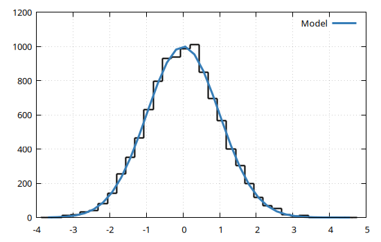

A similar problem in 2D can be handled as follows:

using Random, GModelFit, Gnuplot

# Calculate histogram of the distribution
hh = hist(1 .+ randn(10000), 2 .* randn(10000))

# Define domain and data and fit a model
dom = CartesianDomain(hist_bins(hh, 1), hist_bins(hh, 2))
data = Measures(dom, hist_weights(hh) .* 1., 1.)
model = Model(GModelFit.Gaussian(1e3, 0, 0, 1, 1, 0))
bestfit, stats = fit(model, data)

(Components:
╭───────────┬─────────────┬───────┬─────────────┬───────────┬───────────┬───────────┬─────────╮
│ Component │ Type        │ #Free │ Eval. count │ Min       │ Max       │ Mean      │ NaN/Inf │
├───────────┼─────────────┼───────┼─────────────┼───────────┼───────────┼───────────┼─────────┤
│ main      │ Gaussian_2D │ 6     │ 171         │ 0.0007026 │     373.5 │     44.48 │ 0       │
╰───────────┴─────────────┴───────┴─────────────┴───────────┴───────────┴───────────┴─────────╯

Parameters:
╭───────────┬─────────────┬─────────┬──────────┬───────────┬───────────┬────────┬───────╮
│ Component │ Type        │ Param.  │ Range    │ Value     │ Uncert.   │ Actual │ Patch │
├───────────┼─────────────┼─────────┼──────────┼───────────┼───────────┼────────┼───────┤
│ main      │ Gaussian_2D │ norm    │ 0:Inf    │      4860 │     36.99 │        │       │
│           │             │ centerX │ -Inf:Inf │     1.016 │  0.007681 │        │       │
│           │             │ centerY │ -Inf:Inf │  -0.01685 │   0.01558 │        │       │
│           │             │ sigmaX  │ 0:Inf    │     2.048 │   0.01559 │        │       │
│           │             │ sigmaY  │ 0:Inf    │     1.009 │  0.007681 │        │       │
│           │             │ angle   │ -Inf:Inf │    -90.61 │    0.4013 │        │       │
╰───────────┴─────────────┴─────────┴──────────┴───────────┴───────────┴────────┴───────╯
, Fit results: #data: 225, #free pars: 6, red. fit stat.:     54.314, Status: OK      
)

FComp

As anticipated in Basic concepts and data types any Julia function can be used as a component to evaluate. The corresponding component type is FComp, whose constructors are defined as follows:

FComp(funct::Function, deps=Symbol[]; par1=guess1, par2=guess2, ...)
FComp(funct::FunctDesc)

In the first constructor funct is the Julia function, deps is a vector of dependencies (either the domain dimensions or other component names) and par1, par2 etc. are the named parameters with their corresponding initial guess values.

Example

using GModelFit

# Define a simple Julia function to evaluate a linear relationship
myfunc(x, b, m) = b .+ x .* m

# Define a model with a `FComp` wrapping the previously defined function.
# Also specify the initial guess parameters.
model = Model(:linear => GModelFit.FComp(myfunc, [:x], b=2, m=0.5))

# Fit model against a data set
data = Measures([4.01, 7.58, 12.13, 19.78, 29.04], 0.4)
bestfit, stats = fit(model, data)

(Components:
╭───────────┬───────┬───────┬─────────────┬───────────┬───────────┬───────────┬─────────╮
│ Component │ Type  │ #Free │ Eval. count │ Min       │ Max       │ Mean      │ NaN/Inf │
├───────────┼───────┼───────┼─────────────┼───────────┼───────────┼───────────┼─────────┤
│ linear    │ FComp │ 2     │ 53          │     2.056 │     26.96 │     14.51 │ 0       │
╰───────────┴───────┴───────┴─────────────┴───────────┴───────────┴───────────┴─────────╯

Parameters:
╭───────────┬───────┬────────┬──────────┬───────────┬───────────┬────────┬───────╮
│ Component │ Type  │ Param. │ Range    │ Value     │ Uncert.   │ Actual │ Patch │
├───────────┼───────┼────────┼──────────┼───────────┼───────────┼────────┼───────┤
│ linear    │ FComp │ b      │ -Inf:Inf │     -4.17 │     2.361 │        │       │
│           │       │ m      │ -Inf:Inf │     6.226 │    0.7119 │        │       │
╰───────────┴───────┴────────┴──────────┴───────────┴───────────┴────────┴───────╯
, Fit results: #data: 5, #free pars: 2, red. fit stat.:     31.671, Status: OK      
)

In the second constructor a GModelFit.FunctDesc object is accepted, as generated by the @fd macro). The function is typically a mathematical expression combining any number of parameters and/or other component evaluations within the same model. The expression should be given in the form:

@fd (x, [y, [further domain dimensions...],]
    [comp1, [comp2, [further components ...],]]
    [par1=guess1, [par2=guess2, [further parameters]]]) ->
    (mathematical expression)

where the mathematical expression returns a Vector{Float64} with the same length as the model domain.

The previous example can be rewritten as follows:

using GModelFit

# Define a linear model (with initial guess parameters)
model = Model(:linear => @fd (x, b=2, m=0.5) -> (b .+ x .* m))

# Fit model against data
data = Measures([4.01, 7.58, 12.13, 19.78, 29.04], 0.4)
bestfit, stats = fit(model, data)

(Components:
╭───────────┬───────┬───────┬─────────────┬───────────┬───────────┬───────────┬─────────╮
│ Component │ Type  │ #Free │ Eval. count │ Min       │ Max       │ Mean      │ NaN/Inf │
├───────────┼───────┼───────┼─────────────┼───────────┼───────────┼───────────┼─────────┤
│ linear    │ FComp │ 2     │ 53          │     2.056 │     26.96 │     14.51 │ 0       │
╰───────────┴───────┴───────┴─────────────┴───────────┴───────────┴───────────┴─────────╯

Parameters:
╭───────────┬───────┬────────┬──────────┬───────────┬───────────┬────────┬───────╮
│ Component │ Type  │ Param. │ Range    │ Value     │ Uncert.   │ Actual │ Patch │
├───────────┼───────┼────────┼──────────┼───────────┼───────────┼────────┼───────┤
│ linear    │ FComp │ b      │ -Inf:Inf │     -4.17 │     2.361 │        │       │
│           │       │ m      │ -Inf:Inf │     6.226 │    0.7119 │        │       │
╰───────────┴───────┴────────┴──────────┴───────────┴───────────┴────────┴───────╯
, Fit results: #data: 5, #free pars: 2, red. fit stat.:     31.671, Status: OK      
)

Note that a FComp component can be added to a model without explicitly invoking its constructor when the @fd macro is used.

The evaluation of a FComp component may also involve the outcomes from other components. Continuing from previous example, whose fit was clearly a poor one, we may add a quadratic term to the previously defined linear component:

model[:quadratic] = @fd (x, linear, p2=1) -> (linear .+ p2 .* x.^2)
bestfit, stats = fit(model, data)

(Components:
╭───────────┬───────┬───────┬─────────────┬───────────┬───────────┬───────────┬─────────╮
│ Component │ Type  │ #Free │ Eval. count │ Min       │ Max       │ Mean      │ NaN/Inf │
├───────────┼───────┼───────┼─────────────┼───────────┼───────────┼───────────┼─────────┤
│ quadratic │ FComp │ 1     │ 77          │     4.125 │     29.03 │     14.51 │ 0       │
│ └─╴linear │ FComp │ 2     │ 77          │      3.09 │     3.171 │     3.131 │ 0       │
╰───────────┴───────┴───────┴─────────────┴───────────┴───────────┴───────────┴─────────╯

Parameters:
╭───────────┬───────┬────────┬──────────┬───────────┬───────────┬────────┬───────╮
│ Component │ Type  │ Param. │ Range    │ Value     │ Uncert.   │ Actual │ Patch │
├───────────┼───────┼────────┼──────────┼───────────┼───────────┼────────┼───────┤
│ linear    │ FComp │ b      │ -Inf:Inf │      3.07 │    0.7208 │        │       │
│           │       │ m      │ -Inf:Inf │   0.02029 │    0.5493 │        │       │
├───────────┼───────┼────────┼──────────┼───────────┼───────────┼────────┼───────┤
│ quadratic │ FComp │ p2     │ -Inf:Inf │     1.034 │   0.08981 │        │       │
╰───────────┴───────┴────────┴──────────┴───────────┴───────────┴────────┴───────╯
, Fit results: #data: 5, #free pars: 3, red. fit stat.:    0.70582, Status: OK      
)

The keywords given when defining the function are interpreted as component parameters, hence their properties can be retrieved with:

println("Best fit values:")
println("b:  ", bestfit[:linear].b.val    , " ± ", bestfit[:linear].b.unc)
println("m:  ", bestfit[:linear].m.val    , " ± ", bestfit[:linear].m.unc)
println("p2: ", bestfit[:quadratic].p2.val, " ± ", bestfit[:quadratic].p2.unc)

Best fit values:
b:  3.0699999992111633 ± 0.7207527811763804
m:  0.02028571492419867 ± 0.5492615451533973
p2: 1.0342857141828363 ± 0.0898138664922902

FCompv

Just like FComp, also FCompv is a wrapper for a standard Julia function whose evaluation is performed using the function itself. However, FCompv parameters are passed to the function as a single vector of floats. The FCompv constructors are defined as follows:

FComp(funct::Function, guess::Vector{Float64})
FComp(funct::Function, deps::Vector{Symbol}, guess::Vector{Float64})

where funct is the Julia function, deps is an optional vector of dependencies (either the domain dimensions or other component names) and guess is a vector of initial guess values.

Example

The following example shows how to estimate the vector x satisfying the linear equation Ax = b, where A and b are:

A = [1.43  2.17 -0.38
     0.21 -0.33 -1.71
    -1.23 -1.16  0.83
    -2.09  0.44  0.64]
b = [3.14, -8.48, 0.53, 0.54]

To define the model we will rewrite the equation as Ax - b = 0, and define a model as follows

model = Model(GModelFit.FCompv(x -> A*x - b,
                               [1, 1, 1]))

where x = [1, 1, 1] are the initial guess values for the three parameters in the fit. In this case the empirical data to compare the model to are just zeros, and we will assume a constant uncertainty of 1 for all samples:

data = Measures(fill(0., length(b)), 1.)
bestfit, stats = fit(model, data)

(Components:
╭───────────┬────────┬───────┬─────────────┬───────────┬───────────┬───────────┬─────────╮
│ Component │ Type   │ #Free │ Eval. count │ Min       │ Max       │ Mean      │ NaN/Inf │
├───────────┼────────┼───────┼─────────────┼───────────┼───────────┼───────────┼─────────┤
│ main      │ FCompv │ 3     │ 57          │  -0.01477 │    0.1038 │   0.04577 │ 0       │
╰───────────┴────────┴───────┴─────────────┴───────────┴───────────┴───────────┴─────────╯

Parameters:
╭───────────┬────────┬────────┬──────────┬───────────┬───────────┬────────┬───────╮
│ Component │ Type   │ Param. │ Range    │ Value     │ Uncert.   │ Actual │ Patch │
├───────────┼────────┼────────┼──────────┼───────────┼───────────┼────────┼───────┤
│ main      │ FCompv │ p1     │ -Inf:Inf │      1.52 │   0.06207 │        │       │
│           │        │ p2     │ -Inf:Inf │     1.328 │   0.05828 │        │       │
│           │        │ p3     │ -Inf:Inf │     4.871 │   0.07574 │        │       │
╰───────────┴────────┴────────┴──────────┴───────────┴───────────┴────────┴───────╯
, Fit results: #data: 4, #free pars: 3, red. fit stat.:   0.015942, Status: OK      
)

SumReducer

A component calculating the element-wise sum of a number of other components.

The SumReducer constructor is defined as follows:

SumReducer(args::AbstractSet{Symbol})
SumReducer(args::Vector{Symbol})
SumReducer(args::Vararg{Symbol})

where the Symbols represent the component names

The SumReducer component has no parameter.

Example

using GModelFit

# Define domain and a linear model (with initial guess parameters)
model = Model(:linear => @fd (x, b=2, m=0.5) -> (b .+ x .* m))

# Add a quadratic component to the model
model[:quadratic] = @fd (x, p2=1) -> (p2 .* x.^2)

# The total model is the sum of `linear` and `quadratic`
model[:main] = SumReducer(:linear, :quadratic)

# Fit model against data
dom = Domain(1:5)
data = Measures(dom, [4.01, 7.58, 12.13, 19.78, 29.04], 0.4)
bestfit, stats = fit(model, data)

(Components:
╭──────────────┬────────────┬───────┬─────────────┬───────────┬───────────┬───────────┬─────────╮
│ Component    │ Type       │ #Free │ Eval. count │ Min       │ Max       │ Mean      │ NaN/Inf │
├──────────────┼────────────┼───────┼─────────────┼───────────┼───────────┼───────────┼─────────┤
│ main         │ SumReducer │       │ 77          │     4.125 │     29.03 │     14.51 │ 0       │
│ ├─╴linear    │ FComp      │ 2     │ 77          │      3.09 │     3.171 │     3.131 │ 0       │
│ └─╴quadratic │ FComp      │ 1     │ 77          │     1.034 │     25.86 │     11.38 │ 0       │
╰──────────────┴────────────┴───────┴─────────────┴───────────┴───────────┴───────────┴─────────╯

Parameters:
╭───────────┬───────┬────────┬──────────┬───────────┬───────────┬────────┬───────╮
│ Component │ Type  │ Param. │ Range    │ Value     │ Uncert.   │ Actual │ Patch │
├───────────┼───────┼────────┼──────────┼───────────┼───────────┼────────┼───────┤
│ linear    │ FComp │ b      │ -Inf:Inf │      3.07 │    0.7208 │        │       │
│           │       │ m      │ -Inf:Inf │   0.02029 │    0.5493 │        │       │
├───────────┼───────┼────────┼──────────┼───────────┼───────────┼────────┼───────┤
│ quadratic │ FComp │ p2     │ -Inf:Inf │     1.034 │   0.08981 │        │       │
╰───────────┴───────┴────────┴──────────┴───────────┴───────────┴────────┴───────╯
, Fit results: #data: 5, #free pars: 3, red. fit stat.:    0.70582, Status: OK      
)