Miscellaneous

Generate mock datasets

In some case it is useful to test a model for robustness before the emprical data are available for fitting. This can be achieved via the GModelFit.mock() function, whose purpose is to generate a mock dataset which simulates a measurement process by adding random noise to the foreseen ground-truth.

Example

using GModelFit

model = Model(:main => @fd (x, T=3.14) -> sin.(x ./ T) ./ (x ./ T))

# Generate a mock dataset on a specific domain
dom = Domain(1:0.1:50)
data = GModelFit.mock(Measures, model, dom, seed=1)

# Fit model against the mock dataset
bestfit, fsumm = fit(model, data)

(Components:
╭───────────┬───────┬───────┬─────────────┬───────────┬───────────┬───────────┬─────────╮
│ Component │ Type  │ #Free │ Eval. count │    Min    │    Max    │   Mean    │ NaN/Inf │
├───────────┼───────┼───────┼─────────────┼───────────┼───────────┼───────────┼─────────┤
│ main      │ FComp │ 1     │ 23          │   -0.2172 │    0.9832 │   0.08517 │ 0       │
╰───────────┴───────┴───────┴─────────────┴───────────┴───────────┴───────────┴─────────╯

Parameters:
╭───────────┬───────┬────────┬──────────┬───────────┬───────────┬────────┬───────╮
│ Component │ Type  │ Param. │  Range   │   Value   │  Uncert.  │ Actual │ Patch │
├───────────┼───────┼────────┼──────────┼───────────┼───────────┼────────┼───────┤
│ main      │ FComp │ T      │ -Inf:Inf │     3.141 │   0.01238 │        │       │
╰───────────┴───────┴────────┴──────────┴───────────┴───────────┴────────┴───────╯
, Fit summary: #data: 491, #free pars: 1, red. fit stat.: 1.0596, status: OK      
)

Serialization

A few structures, namely GModelFit.ModelSnapshot, GModelFit.FitSummary and Measures{N}, as well as Vector(s) of such structures can be serialized, i.e. stored in a JSON file using TypedJSON.jl. The structures can later be de-serialized in a separata Julia session without the need to re-run the fitting process used to create them in the first place.

Example

In the following we will generate a few GModelFit.jl objects and serialized them in a file.

using GModelFit, TypedJSON

dom = Domain(1:0.1:50)
model = Model(:main => @fd (x, T=3.14) -> sin.(x ./ T) ./ (x ./ T))
data = GModelFit.mock(Measures, model, dom, seed=1)
bestfit, fsumm = fit(model, data)

# Serialize objects and save in a file
TypedJSON.serialize("save_for_future_use.json", (bestfit, fsumm, data))

The same objects can be de-serialized in a different Julia session:

using GModelFit, TypedJSON
bestfit, fsumm, data = TypedJSON.deserialize("save_for_future_use.json")

(Components:
╭───────────┬───────┬───────┬─────────────┬───────────┬───────────┬───────────┬─────────╮
│ Component │ Type  │ #Free │ Eval. count │    Min    │    Max    │   Mean    │ NaN/Inf │
├───────────┼───────┼───────┼─────────────┼───────────┼───────────┼───────────┼─────────┤
│ main      │ FComp │ 1     │ 23          │   -0.2172 │    0.9832 │   0.08517 │ 0       │
╰───────────┴───────┴───────┴─────────────┴───────────┴───────────┴───────────┴─────────╯

Parameters:
╭───────────┬───────┬────────┬──────────┬───────────┬───────────┬────────┬───────╮
│ Component │ Type  │ Param. │  Range   │   Value   │  Uncert.  │ Actual │ Patch │
├───────────┼───────┼────────┼──────────┼───────────┼───────────┼────────┼───────┤
│ main      │ FComp │ T      │ -Inf:Inf │     3.141 │   0.01238 │        │       │
╰───────────┴───────┴────────┴──────────┴───────────┴───────────┴────────┴───────╯
, Fit summary: #data: 491, #free pars: 1, red. fit stat.: 1.0596, status: OK      
, Measures{1}: (length: 491)
╭─────────┬───────────┬───────────┬───────────┬───────────┬───────────┬─────────╮
│         │    Min    │    Max    │   Mean    │  Median   │ Std. dev. │ Nan/Inf │
├─────────┼───────────┼───────────┼───────────┼───────────┼───────────┼─────────┤
│ values  │   -0.3439 │       1.1 │   0.08667 │   0.02283 │    0.2741 │         │
│ uncerts │   0.06002 │   0.06985 │   0.06166 │   0.06082 │   0.00229 │         │
╰─────────┴───────────┴───────────┴───────────┴───────────┴───────────┴─────────╯
)

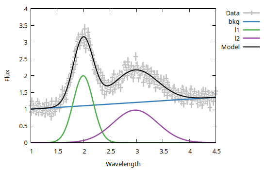
Quick plot (1D)

The GModelFit.jl package implements Gnuplot.jl recipes to display plots of Measures{1} and ModelSnapshot objects., e.g.:

Example

Create a model, a mock dataset and run a fit:

using GModelFit

dom = Domain(0:0.01:5)
model = Model(:bkg => GModelFit.OffsetSlope(1, 1, 0.1),
              :l1 => GModelFit.Gaussian(1, 2, 0.2),
              :l2 => GModelFit.Gaussian(1, 3, 0.4),
              :main => SumReducer(:bkg, :l1, :l2))
data = GModelFit.mock(Measures, model, dom)
bestfit, fsumm = fit(model, data)

A plot of the dataset and of the best fit model can be simply obtained with

using Gnuplot
@gp data bestfit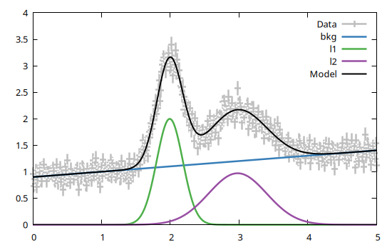

You may also specify axis range, labels, title, etc. using the standard Gnuplot.jl keyword syntax, e.g.:

using Gnuplot
@gp xr=[1, 4.5] xlabel="Wavelength" ylab="Flux" "set key outside" data bestfit