Plot recipes

A plot recipe is a quicklook visualization procedure aimed at reducing the amount of repetitive code to generate a plot. More specifically, a recipe is a function that convert the plot specs from the "Julia world" into a form suitable to be ingested in gnuplot, namely a Vector{<: AbstractGPSpec}) (see also Gnuplot.jl internals). The latter contain informations on how to create a plot, or a part of it, and can be used directly as arguments in a @gp or @gsp call.

There are two kinds of recipes:

explicit recipe: a function which is explicitly invoked by the user. It can have any name and accept any number of arguments and keywords. It is typically used when the visualization of a data type requires some extra information, beside data itself (e.g. to plot data from a DataFrame object, see Simple explicit recipe);
implicit recipe: a function which is automatically called by Gnuplot.jl. It must extend the Gnuplot.recipe() function, and accept exactly one mandatory argument. It is typically used when the visualization is completely determined by the data type itself (e.g. the visualization of a Matrix{ColorTypes.RGB} object as an image, see Image recipes);

An implicit recipe is invoked whenever the data type of an argument to @gp or @gsp is not among the allowed ones (see Gnuplot.parseSpecs documentation). If a suitable recipe do not exists an error is raised. On the other hand, an explicit recipe needs to be invoked by the user, and the output passed directly to @gp or @gsp.

Although recipes provides very efficient tools for data exploration, their use typically hide the details of plot generation. As a consequence they provide less flexibility than the approaches described in Basic usage and Advanced usage.

Currently, the Gnuplot.jl package provides only one explicit recipe (line()) and a few implicit ones. All recipes are implemented in recipes.jl.

Simple explicit recipe

To generate a plot using the data contained in a DataFrame object we need, beside the data itself, the name of the columns to use for the X and Y coordinates. The following example shows how to implement an explicit recipe to plot a DataFrame object:

using RDatasets, DataFrames, Gnuplot

function plotdf(df::DataFrame, colx::Symbol, coly::Symbol; group=nothing)
    if isnothing(group)
        return Gnuplot.parseSpecs(df[:, colx], df[:, coly], "w p notit",
                                  xlab=string(colx), ylab=string(coly))
    end

    out = Vector{Gnuplot.AbstractGPSpec}()
	append!(out, Gnuplot.parseSpecs(xlab=string(colx), ylab=string(coly)))
    for g in sort(unique(df[:, group]))
        i = findall(df[:, group] .== g)
        if length(i) > 0
            append!(out, Gnuplot.parseSpecs(df[i, colx], df[i, coly], "w p t '$g'"))
        end
    end
    return out
end

# Load a DataFrame and plot two of its columns
iris = dataset("datasets", "iris")
@gp plotdf(iris, :SepalLength, :SepalWidth, group=:Species)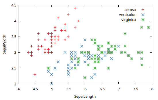

Corner plot recipe

The following is a slightly more complex example illustrating how to generate a corner plot:

using RDatasets, DataFrames, Gnuplot

function cornerplot(df::DataFrame; nbins=5, margins="0.1, 0.9, 0.15, 0.9", spacing=0.01, ticscale=1)
    numeric_cols = findall([eltype(df[:, i]) <: Real for i in 1:ncol(df)])
    out = Vector{Gnuplot.AbstractGPSpec}()
    append!(out, Gnuplot.parseSpecs("set multiplot layout $(length(numeric_cols)), $(length(numeric_cols)) margins $margins spacing $spacing columnsfirst downward"))
    id = 1
    for ix in numeric_cols
        for iy in numeric_cols
            append!(out, Gnuplot.parseSpecs(id, xlab="", ylab="", "set xtics format ''", "set ytics format ''", "set tics scale $ticscale"))
            (iy == maximum(numeric_cols))  &&  append!(out, Gnuplot.parseSpecs(id, xlab=names(df)[ix], "set xtics format '% h'"))
            (ix == minimum(numeric_cols))  &&  append!(out, Gnuplot.parseSpecs(id, ylab=names(df)[iy]))

            xr = extrema(df[:, ix])
            yr = extrema(df[:, iy])
            if ix == iy
                h = hist(df[:, ix], range=xr, nbins=nbins)
                append!(out, Gnuplot.parseSpecs(id, "unset ytics", xr=xr, yr=[NaN,NaN], hist_bins(h), hist_weights(h), "w steps notit lc rgb 'black'"))
            elseif ix < iy
                append!(out, Gnuplot.parseSpecs(id,                xr=xr, yr=yr       , df[:, ix], df[:, iy], "w p notit"))
            else
                append!(out, Gnuplot.parseSpecs(id, "set multiplot next"))  # skip slot
            end
            id += 1
        end
    end
    return out
end

# Load a DataFrame and generate a cornerplot
iris = dataset("datasets", "iris")
@gp cornerplot(iris)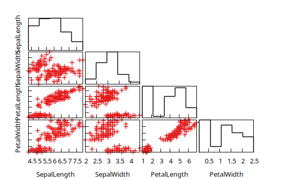

Histogram recipes

The object returned by the hist() function can be readily visualized by means of implicit recipes defined on the StatsBase.Histogram type (in both 1D and 2D) types:

x = randn(1000);
@gp hist(x)

x = randn(10_000);
y = randn(10_000);
@gp hist(x, y)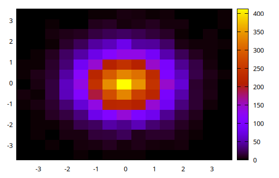

Contour lines recipes

The object returned by the contourlines() function can be readily visualized by means of implicit recipes defined on the Gnuplot.IsoContourLines types:

x = randn(10_000);
y = randn(10_000);
h = hist(x, y)
clines = contourlines(h, "levels discrete 10, 30, 60, 90");
@gp clines

Image recipes

The Gnuplot.jl package provides implicit recipes to display images in the following formats:

Matrix{ColorTypes.RGB{T}};
Matrix{ColorTypes.RGBA{T}}
Matrix{ColorTypes.Gray{T}};
Matrix{ColorTypes.GrayA{T}};

To use these recipes simply pass an image to @gp, e.g.:

using TestImages
img = testimage("lighthouse");
@gp img

All such recipes are defined as:

function recipe(M::Matrix{ColorTypes.RGB{T}}, opt="flipy")
  ...
end

with only one mandatory argument. In order to exploit the optional keyword we can explicitly invoke the recipe as follows:

img = testimage("walkbridge");
@gp palette(:gray1) Gnuplot.recipe(img, "flipy rot=15deg")

Note that we used both a palette (:gray, see Palettes and line types) and a custom rotation angle.

The flipy option is necessary for proper visualization (see discussion in Plot matrix as images).